2.7. MedeA Flowcharts: Design and Automate Simulation Workflows
Contents
| download: | pdf |
|---|
The MedeA environment provides graphical flowcharts to support the efficient construction of complex computational protocols. These flowcharts can be easily created to describe and control the flow of calculations, allowing simple and straightforward access to the various computation engines of MedeA, such as LAMMPS, GIBBS, VASP, MOPAC and Gaussian. These different engines may be combined within a single flowchart, so that a VASP optimization of a unit cell, for example, may be employed as a prelude to a larger scale LAMMPS simulation using an embedded atom method (EAM) forcefield. In addition, the structure can be modified within the flowchart using the provided building and editing capabilities.
The backbone of the flowchart infrastructure is the Tcl language (see https://www.tcl.tk/) which can be directly accessed within custom-scripting stages. Once created the flowcharts can be saved as ASCII files allowing them to be reused and distributed.
Although flowcharts are customizable and flexible their use is straightforward. In this section the basic concepts are summarized, allowing for the construction of both simple and complex flowcharts. Additional details for specific tools are provided elsewhere within the MedeA User’s Guide.
2.7.1. Flowcharts Overview
Flowcharts are accessed via the Jobs >> New Job… menu item. This command yields the main flowchart user interface, where flowcharts are constructed, read from disk or previous calculations or saved to the disk.
Flowcharts provide a variety of control capabilities, such as a While Loop, For Loop, Foreach Structure Loop, If and Foreach Loop. This allows for considerable flexibility in the automation of simulations. For example, a scan of possible system temperatures and pressures for molecular dynamics calculations may be achieved with nested Foreach loops.
Additionally, custom Tcl scripting may be included in a flowchart. Key results from simulation stages are available as variables, which can be operated on, tabulated, and also used to control subsequent stages, allowing the convenient construction of highly automated procedures for selected applications. If more complex manipulation of the results are required, a custom Tcl stage can be used to process the outputs of the current and any previous stages.

Materials Design flowcharts begin with the Start command which is automatically placed on the left-hand panel of the flowchart dialog. Typically after the Start stage, several variables will be set using a Set Variables stage. The stage is added to the flowchart by clicking the Set Variables button on the right-hand panel.
In general, stages are added to a flowchart by clicking the appropriate element on the right-hand pane of the flowchart dialog or user interface. Once added to a flowchart, most stages may be edited by either right-clicking that element and selecting Edit, or double-clicking on that stage.
A summary of the functionality and use of specific flowchart elements is provided below.
2.7.2. Initialization and Control
This section of the flowchart interface provides the following stages: Subchart, Set Variables, Print Variables, Custom Tcl Script, and loop related commands: For Loop, Foreach Loop, While Loop, Foreach Structure Loop, Catch and If.
As discussed above, every flowchart begins with a Start stage, this is employed as the starting point of execution for the flowchart and is automatically included in the flowchart. The Subchart stage is simply a container that can hold other flowcharts. This provides a convenient way to break up a large more complicated flowchart into simpler parts and provides a simple way to include a previous flowchart as a building block into a more complicated protocol.
The Set Variables stage allows the user to set the value and units of specific variables that will be employed in later stages in the flowchart. For example, the Set Variables stage can be used to set:
| Variable | Value | Unit |
| T | 300 | K |
| tstep | 1 | fs |
| P | 1 | atm |
These variables will then be used throughout subsequent stages in LAMMPS
calculations, which employ T, tstep, and P as default variables for
temperature, timestep, and pressure, respectively. This centralization of
the variable setting is convenient in exploring the effect of the system
variables on simulated properties.
Once declared variables can be accessed, following the Tcl paradigm,
by adding a $ sign in front of the variable name, for example, the variable tstep can
be accessed with $tstep.
The Print Variables reports (calculated) variables matching a specific name, including variables created and made accessible by any previous stage. These variables can be printed to tables or added to structure lists.
The Custom Tcl Script allows you to enter, or retrieve from a file Tcl commands (see https://www.tcl.tk/) which may be used to carry out specific actions during the execution of a flowchart. This can be useful in preparing result summaries or in determining whether specific simulation conditions have been met.
The For Loop includes a flowchart executed repeatedly as defined by the control variables and test conditions.
The Foreach Loop and While Loop stages allow for the
introduction of control structures within a flowchart. In each case,
allowing for the introduction of a complete flowchart to be executed
repeatedly until the foreach vector (like {T, P}) of variables is
exhausted, or the while condition is no longer true.
The Foreach Structure Loop takes structures contained in a Structures List or a previous Trajectory and performs on each of these structures the same calculation protocol as defined in the Foreach Structure Loop flowchart. This stage is part of the MedeA HT-Launchpad module.
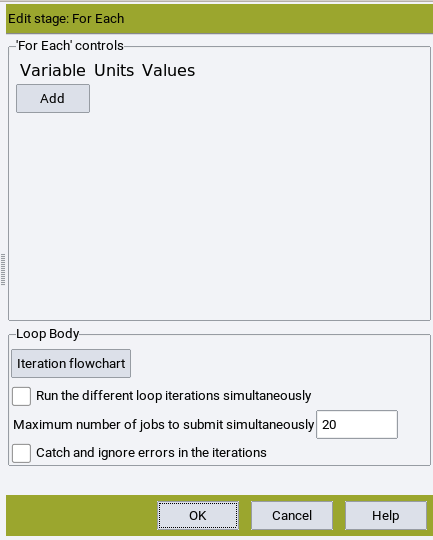
Stages within the loops are executed either sequentially, meaning that each iteration is completed before the next is started, or simultaneously, where multiple iterations run in parallel. The simultaneous operation mode can be switched on by checking Run the different loop iterations simultaneously, specifying the degree of parallel operation by the parameter Maximum number of jobs to submit simultaneously. All looping structures have an option to Catch and ignore errors in the iterations.
The Catch stage allows for more elaborate error handling, that is in case the flowchart runs into an error, it is caught and another flowchart is executed.
The If stage allows execution of a flowchart if a condition is true (then), or an alternative flowchart (else).
2.7.3. Tables and Graphs
This section allows defining a Table, insert results as soon as they occur with Add Row, and finally Print the entire table. The flowchart below is just an illustration, leaving out all looping and calculation.

With Table you define a Table by giving it a name and adding columns. Each column has a
Title:Name of the column
Units: Results are converted into units chosen. If no unit is specified, the default unit is used.
Justification: Left, right, or center
Width: How much “space” on the left and right
Format: Can be provided in the printf format. For example;%#dor%#ifor integer values,%#.#ffor float/double values,%#cfor characters,%#sfor strings, and%#xfor hexadecimal values.Hint
The maximum number of characters/digits that can be used to print a given variable can be defined by an integer value
#between the%sign and the character. In the case of a float value two numbers, separated by a comma, can be used. In this case, the second number defines the number of digits after the comma used to print the value. For example,%8.2fdisplays a floating-point variable with up to 8 characters in total and two digits after the comma.
Table: Add Row adds a line of results to a specified table. Variables can be added,
following the Tcl paradigm, by adding a $ sign in front of the variables name,
e.g., the variable Etotal_calc can be printed with $Etotal_calc into a table.
See Available Variables for a list of available variables that can be added.
Table: Print the selected Table. You can also save or
append the result to a file as formatted text,
comma separated values (csv), tab-delimited,
or delimited by a different Separator like ;.
2.7.4. General Properties
Hill-Walpole bounds: applies Hill-Walpole statistics on top of Mechanical Properties (see the section on Hill-Walpole bounds for amorphous systems).
Mechanical Properties determines the mechanical properties with LAMMPS or VASP based on given Strains. For more information refer to the chapter on the Theory of elasticity.
Deformation performs deformation simulations beyond the elastic regime with LAMMPS or VASP. For more information refer to the MedeA Deformation section.
Effective Mass: uses VASP to determine the effective mass for a specified k-point. For a more detailed description of the use of this stage see the section on Accurate Effective Mass calculations.
2.7.5. Methods
The Methods section of the flowchart interface provides access to a computational engine such as GIBBS, LAMMPS, MOPAC, GAUSSIAN or VASP (VASP flowcharts or a stage accessing the VASP GUI otherwise accessible from the Tools menu). In each case, the interface provided allows you to start a new flowchart and execute relevant specific commands within this new flowchart.
In addition, there are methods available making use of the computational engines above to calculate vibrational properties, phonon dispersion, and phonon density of states (Phonon), to optimize cluster expansions for alloys and other disordered systems and perform Monte Carlo simulations for larger ensembles (UNCLE), to predict properties of polymers using correlations (P3C) or group contributions (QSPR), and to optimize force field parameters by fitting to ab initio data (Forcefield Optimizer and MLP Generator).
Additional information on each of the Methods available in this section of the flowchart interface is available in the section of the User’s Guide dealing with each method.
2.7.6. Building and Editing
Flowchart building commands allow for the construction and adjustment of atomic models.
2.7.6.1. Set Cell
The Set Cell stage permits the adjustment of unit cell dimensions for periodic systems. Here a variety of options are supported, the density or volume may be specified, or an expansion factor applied to the current system, or specific unit cell dimensions set. This stage may be combined with an appropriate Foreach Loop to explore the volumetric or density-specific behavior of a given system property.
2.7.6.2. Change periodicity
A stage to turn on or remove periodic boundary conditions. In this stage the specify a gap to leave between the periodic building blocks. This stage may be used to combine a non-periodic calculation, for example with MOPAC, with a periodic VASP calculation.
2.7.6.3. Supercell
The Supercell command may be applied to increase the size of a given model. As this building process is executed on the JobServer this is an efficient mechanism to create large systems.
2.7.6.4. Amorphous builder
The Amorphous Builder stage can be used to create amorphous models. System composition source can be set to the current system, where the current structure is split into molecules and recombined, to composition files saved on the local machine, and to a composition used in a previous job with jobserver. The system geometry of the amorphous material can be either bulk cell or layer and is build according to the set Temperature and cell dimensions. The latter is set with specify cell and can be a mixture of the specific cell dimensions a, b, and c in combination with density. Accordingly, additional options become available. The number of mols of the defined composition is set with Nmols. As this is a stochastic process the number of configurations that is to be created can be set. Multiple amorphous structures can be used to determine the average property of a given model. See the section on Amorphous Materials Builder for more information.
2.7.6.5. Thermoset Builder
The Thermoset Builder creates a single configuration of a densely crosslinked thermoset structure from an equilibrated bulk amorphous system. See the section on Thermoset Builder for more information.
2.7.6.6. Translate Atoms
The Translate Atoms command can be used to adjust the position of atoms within the current system. Thereby it is possible to explicitly select atoms of the active structure or to select a subset. Atoms can be translated by a translation vector or to a point. The displacement can be in fractional or cartesian coordinates.
2.7.6.7. Docking
The Docking stage combines two structures. The host structure is the ‘stream’ structure upon which the Flowchart is operating. The Guest from Job is specified as the final.sci of the specified job on the current Job Server, the Host is specified as the input structure submitted with the flowchart. Number of guests defines how many guest molecules are put into the host, for each guest this process is repeated for Maximum iterations. The Maximum displacement (Ang) should be larger than the diameter of any ring to avoid the interlocking of molecules. Scale rotations by and Temperature (K), as well as the underlying theory, is explained in the section on Docking.
2.7.6.8. Randomly Substitute Atoms
Replaces a defined number of atoms, accounting for the symmetry of the structure, of element A with either vacancies or atoms of element B. For more information refer to the section on Random Substitution.
2.7.6.9. Simple Dynamics & Minimization
This stage uses the same simple dynamics and minimization algorithm that is also accessible from the MedeA GUI. The Number of dynamics steps and the Number of minimization steps can be set separately. Use this stage to pre-optimize a structure before applying a computationally more demanding algorithm to it.
2.7.6.10. Subset Manager
Manipulate existing subsets in a structure.
2.7.7. Structures Lists
These are a collection of commands to handle Structures Lists:
New List creates a new structure list that is accessible by the current flowchart. The List name and the File name of the structure lists can be defined. If no subfolder is specified the list will be placed in the job folder. The list can be initialized from an initial list that is saved locally on the machine running the MedeA GUI. Note, that multiple structure lists can be active at the same time.
Save to List adds the current structure to any of the active structure lists. In addition, the structure can be saved with multiple properties.
Extract from List will extract a structure, specified by Structure index and Configuration index, from any of the active lists.
Sort List will sort any of the active structure lists according to a specific property.
Remove Duplicates from List remove all duplicates from a given list. Duplicates are identified by making use of symmetry.
Compute Descriptors on a list define and compute descriptors on a list.
Apply QSAR model on a List by loading the equation from an XML QSAR model file.
For more details, please see the MedeA High-Throughput section.
Documentation_HT
2.7.8. Forcefield
Set Forcefield allows you to specify a forcefield.
Assign Atom Types and Charges allows you to readjust or set atomic forcefield parameters. This requires a forcefield with auto-typing.
2.7.9. Analysis
Orientation determines the orientation of a subset to a given reference vector:(x, y, or z).
2.7.10. Available Variables
Properties listed below are made available in the flowchart after a specified stage as variables.
To access the value of any of these variables use a $ sign in front of the property name.
For example, the value of the variable Etotal_calc can be accessed with $Etotal_calc.
2.7.10.1. Structure-Specific Properties
Different properties of structures (systems) are available through variables without
performing any calculation. The name of the active system can be accessed with
$system_name.
| Property | Unit | Description |
|---|---|---|
| system_name | none | name of the active system |
Values of the properties listed in the below table can change after calculations, i.e.
can be different prior and after calculations are performed.
The syntax to access the value of any of the properties is [$system get property], whereby [ and ] is
the Tcl syntax to declare a string in command (see https://www.tcl.tk/), and Property should be replaced
by one of the properties in the below table.
For example, the Tcl command [$system get density] returns the value 1.2345 kg/m^3, i.e.
a number together with a unit.
The Tcl command [$system get cell.a] returns only a single value without a unit but the value is in the unit
of \({\mathring{\mathrm{A}}}\).
| Property | Unit | Description | Remark |
|---|---|---|---|
| density | kg/m3 | mass density | only available for structures with simulation/crystal cells and periodic boundary conditions |
| volume | m3 | volume of conventional simulation/crystal cell | only available for structures with simulation/crystal cells and periodic boundary conditions |
| primitiveCellVolume | m3 | volume of primitive simulation/crystal cell with the space group P1 | only available for structures with simulation/crystal cells and periodic boundary conditions |
| mass | kg | sum of molar atomic masses | available for all structures |
| forcefield_mass | none | sum of atomic masses that are determined by the assigned forcefield parameters | only available for structures with simulation/crystal cells and periodic boundary conditions after forcefield parameters were assigned |
| nAtoms | none | number of constituting atoms | available for all structures |
| nPrimitiveAtoms | none | number of atoms in the primitive cell | only available for structures with simulation/crystal cells and periodic boundary conditions |
| celldata | none | returns a list of the cell parameters in the sequence \(a\), \(b\), \(c\), \(\alpha\), \(\beta\), \(\gamma\) whereby cell lengths are in \({\mathring{\mathrm{A}}}\) and angles in degrees. | only available for structures with simulation/crystal cells and periodic boundary conditions |
| formula | none | returns the total composition of a structure | available for all structures |
| empiricalFormula | none | returns the composition of the basic formula unit (stoichiometric unit) of a structure | available for all structures |
| empiricalRatio | none | returns the number of formula units in a structure that is determined by the ratio of the values of the variables formula and empiricalFormula | available for all structures |
| cell.a | none | returns the value (in \({\mathring{\mathrm{A}}}\)) of the length \(a\) of the simulation cell (crystal structure) | only available for structures with simulation/crystal cells and periodic boundary conditions |
| cell.b | none | returns the value (in \({\mathring{\mathrm{A}}}\)) of the length \(b\) of the simulation cell (crystal structure) | only available for structures with simulation/crystal cells and periodic boundary conditions |
| cell.c | none | returns the value (in \({\mathring{\mathrm{A}}}\)) of the length \(c\) of the simulation cell (crystal structure) | only available for structures with simulation/crystal cells and periodic boundary conditions |
| cell.alpha | none | returns the value (in degree) of the cell angle \(\alpha\) of the simulation cell (crystal structure) | only available for structures with simulation/crystal cells and periodic boundary conditions |
| cell.beta | none | returns the value (in degree) of the cell angle \(\beta\) of the simulation cell (crystal structure) | only available for structures with simulation/crystal cells and periodic boundary conditions |
| cell.gamma | none | returns the value (in degree) of the cell angle \(\gamma\) of the simulation cell (crystal structure) | only available for structures with simulation/crystal cells and periodic boundary conditions |
| charge | none | returns the total charge (number of excess electrons) of a molecular (non-periodic) structure | only available for molecular (non-periodic) structures |
| spinMultiplicity | none | returns the total electronic spin multiplicity of a molecular (non-periodic) structure | only available for molecular (non-periodic) structures |
| beadFamily | none | returns the name of mesoscale forcefield to which the beads of the mesoscale structure belong | available for all mesoscale structures (periodic and non-periodic) |
2.7.10.2. Structure Lists
Values saved with structures in a structure list can be accessed for each entry
in that list using the For Each Structure stage. Within that loop variables are accessed for
the active structure with $system_properties(NAME) where NAME defines the
name of the desired and available property. So, if the variable T has been saved with the
structure then its value can be fetched with $system_properties(T).
2.7.10.3. MedeA LAMMPS
| Property | Unit | Description |
|---|---|---|
| Epot_singlepoint_calc | kJ/mol | calculated potential energy |
| Evdwl_singlepoint_calc | kJ/mol | van der Waals pairwise energy including long-range tail correction, Coulomb interactions and interactions between bonded particles are not included |
| Etail_singlepoint_calc | kJ/mol | van der Waals energy long-range tail correction |
| Eangle_singlepoint_calc | kJ/mol | calculated energy due to angular interactions between three particles that are connected through two bonds |
| Ebond_singlepoint_calc | kJ/mol | calculated energy due interactions between two bonded particles |
| Ecoul_singlepoint_calc | kJ/mol | calculated Coulomb energy due to interactions between charged, non-bonded particles; it is the sum of the short-range Coulomb interaction calculated in real space and long-range Coulomb interaction that is calculated in reciprocal space |
| Edihed_singlepoint_calc | kJ/mol | calculated energy due to torsional (dihedral) interactions between four particles in a row that connected through three bonds |
| Eimpro_singlepoint_calc | kJ/mol | calculated energy due to out-of-plane angles interactions between 4 particles that are connected by three bonds, whereby one particle is bonded to all the other three particles |
| Elong_singlepoint_calc | kJ/mol | long-range k-space energy |
When performing a molecular dynamics simulation the mean value of a property is returned with
{property}_calc and its uncertainty with {property}_uncertainty_calc.
The value of the uncertainty is given in the same unit as the calculated property. In addition,
{property}_converged_calc is returned with the value of 1 if the calculated property has converged during the simulation
otherwise it is returned with the value of 0.
| Property | Unit | Averaged | Description |
|---|---|---|---|
| t_calc | fs | no | total simulation time |
| T_calc | K | yes | calculated mean temperature |
| P_calc | atm | yes | calculated mean pressure |
| V_calc | \({\mathring{\mathrm{A}}}\)3 | yes | calculated mean cell volume |
| rho_calc | g/mL | yes | calculated mean mass density |
| Etotal_calc | kJ/mol | yes | calculated mean total energy, i.e. the sum of potential energy and kinetic energy |
| Epot_calc | kJ/mol | yes | calculated mean potential energy |
| Ekin_calc | kJ/mol | yes | calculated mean kinetic energy |
| Evdw_calc | kJ/mol | yes | calculated mean energy that includes all of the charge-independent energy terms for interactions between particles that are not bonded, such as 3-body interactions of a Tersoff potential and a Stillinger-Weber potential, all charge-independent terms of a COMB3 potential and ReaxFF potential, all contributions of a SNAP forcefield, etc; anything related to Coulomb interactions and interactions between bonded particles are not included |
| Ecoul_calc | kJ/mol | yes | calculated mean Coulomb energy due to interactions between charged, non-bonded particles; it is the sum of the short-range Coulomb interaction calculated in real space and long-range Coulomb interaction that is calculated in reciprocal space |
| Enonbond_calc | kJ/mol | yes | calculated mean energy due to interactions between non-bonded particles, i.e. the sum of the values of Ecoul_calc and Evdw_calc |
| Ebond_calc | kJ/mol | yes | calculated mean energy due interactions between two bonded particles |
| Eangle_calc | kJ/mol | yes | calculated mean energy due to angular interactions between three particles that are connected through two bonds |
| Edihed_calc | kJ/mol | yes | calculated mean energy due to torsional (dihedral) interactions between four particles in a row that connected through three bonds |
| Eimp_calc | kJ/mol | yes | calculated mean energy due to out-of-plane angles interactions between 4 particles that are connected by three bonds, whereby one particle is bonded to all the other three particles |
| Eint_calc | kJ/mol | yes | calculated mean energy due to all interactions between bonded particles, i.e. the sum of Eebond_calc, Eangle_calc, Edihed_calc, and Eimp_calc. |
| a_calc | \({\mathring{\mathrm{A}}}\) | yes | calculated mean lattice parameter \(a\) |
| b_calc | \({\mathring{\mathrm{A}}}\) | yes | calculated mean lattice parameter \(b\) |
| c_calc | \({\mathring{\mathrm{A}}}\) | yes | calculated mean lattice parameter \(c\) |
| alpha_calc | 0 | yes | calculated mean lattice parameter \(\alpha\) |
| beta_calc | 0 | yes | calculated mean lattice parameter \(\beta\) |
| gamma_calc | 0 | yes | calculated mean lattice parameter \(\gamma\) |
| Sxx_calc | atm | yes | calculated mean tensile/compressive stress in \(x\) direction |
| Syy_calc | atm | yes | calculated mean tensile/compressive stress in \(y\) direction |
| Szz_calc | atm | yes | calculated mean tensile/compressive stress in \(z\) direction |
| Syz_calc | atm | yes | calculated mean shear stress in \(y\)-\(z\)-plane |
| Sxz_calc | atm | yes | calculated mean shear stress in \(x\)-\(z\)-plane |
| Sxy_calc | atm | yes | calculated mean shear stress in \(x\)-\(y\)-plane |
| nSteps_calc | none | no | total number of the MD steps |
| Fmax_calc | kJ/mol/\({\mathring{\mathrm{A}}}\) | no | calculated maximum remaining particle force after structure minimization |
| Frms_calc | kJ/mol/\({\mathring{\mathrm{A}}}\) | no | calculated root mean square (RMS) of all particle forces after structure minimization |
Additional properties available when using LAMMPS property modules.
| Property | Unit | Averaged | Description |
|---|---|---|---|
| CED_calc | J/cm3 | yes | calculated mean cohesive energy density |
| CEDvdw_calc | J/cm3 | yes | calculated mean contribution of all non-Coulomb, non-bond interactions to the cohesive energy density |
| CEDcoul_calc | J/cm3 | yes | calculated mean contribution of the Coulomb interactions to the cohesive energy density |
| dHvap (ideal)_calc | kJ/mol | yes | calculated mean enthalpy of vaporization (\(\Delta H_{vap}\)) |
| Property | Unit | Averaged | Description |
|---|---|---|---|
| deltaQ_calc | kJ/mol | no | total amount of heat that is transferred during a reverse non-equilibrium molecular dynamics (RNEMD) simulation that employs the Müller-Plathe approach to calculate the thermal conductivity |
| dQ/dt_calc | kJ/mol/fs | yes | mean heat transfer rate that is computed in a reverse non-equilibrium molecular dynamics (RNEMD) simulation that employs the Müller-Plathe approach to calculate thermal conductivity |
| Property | Unit | Averaged | Description |
|---|---|---|---|
| deltapx_calc | \({\mathring{\mathrm{A}}}\)/fs*g/mol | no | total momentum that is transferred during a reverse non-equilibrium molecular dynamics (RNEMD) simulation that employs the Müller-Plathe approach to calculate shear viscosity |
| dpx/dt_calc | \({\mathring{\mathrm{A}}}\)/fs*g/mol/fs | yes | mean momentum transfer rate that is computed in a reverse non-equilibrium molecular dynamics (RNEMD) simulation that employs the Müller-Plathe approach to calculate shear viscosity |
| Property | Unit | Averaged | Description |
|---|---|---|---|
| D_calc | cm2/s | yes | norm of the calculated self-diffusion coefficient of all atoms |
| D_calc_subset | cm2/s | yes | norm of the calculated self-diffusion coefficient for the atoms of subset “subset” |
| Dx_calc | cm2/s | yes | calculated self-diffusion coefficient along the x-axis of all atoms |
| Dx_calc_subset | cm2/s | yes | calculated self-diffusion coefficient along the x-axis for the atoms of subset “subset” |
| Dy_calc | cm2/s | yes | calculated self-diffusion coefficient along the y-axis of all atoms |
| Dy_calc_subset | cm2/s | yes | calculated self-diffusion coefficient along the y-axis for the atoms of subset “subset” |
| Dz_calc | cm2/s | yes | calculated self-diffusion coefficient along the z-axis of all atoms |
| Dz_calc_subset | cm2/s | yes | calculated self-diffusion coefficient along the z-axis for the atoms of subset “subset” |
| Property | Unit | Averaged | Description |
|---|---|---|---|
| Surface_Tension_calc | mN/m | yes | calculated surface tension |
| Property | Unit | Description |
|---|---|---|
| Evib_calc | kJ/mol | total vibrational internal energy (classical and quantum contributions) |
| Evib_QC_calc | kJ/mol | quantum contributions to total vibrational internal energy |
| Epot_total | kJ/mol | sum of MD potential energy Epot, and the vibrational quantum contributions Evib_QC |
| Avib_calc | kJ/mol | total vibrational Helmholtz free energy (classical and quantum contributions) |
| ZPE_calc | kJ/mol | total vibrational zero point energy |
| SvibT_calc | kJ/mol | total vibrational entropy times temperature |
| Svib_calc | J/K/mol | total vibrational entropy (classical and quantum contributions) |
| Cv_calc | J/K/mol | heat capacity at constant volume |
2.7.10.4. MedeA VASP
Different properties are calculated depending on the type of VASP calculation configured within the VASP stage. Properties listed in the first table are always available after a successful VASP calculation.
| Property | Unit | Description |
|---|---|---|
| Eelectronic_calc | eV | VASP energy (for primitive cell) |
| Eelectronic_conventionalCell_calc | eV | VASP energy (for conventional cell) |
| Eelectronic_empiricalFormula_calc | eV | VASP energy (for empirical formula) |
| Eelectronic_sigma0_calc | eV | VASP energy extrapolated to zero smearing (for primitive cell) |
| Enon-dispersive_calc | eV | VASP energy without van der Waals contribution, if van der Waals forcefield is applied (for primitive cell) |
| EVanderWaals_calc | eV | VASP energy, van der Waals contribution, if van der Waals forcefield is applied (for primitive cell) |
| Forces_calc | eV/Ang | List of atomic forces in Cartesian coordinates |
| Force_max_calc | eV/Ang | Maximum absolute atomic force value |
| FormulaPrimitiveCell_calc | Formula of the primitive cell | |
| FormulaConventionalCell_calc | Formula of the conventional cell | |
| FormulaEmpirical_calc | Empirical formula | |
| FactorEmpiricalToPrimitive_calc | Factor to convert empirical formula to primitive cell formula | |
| FactorEmpiricalToConventional_calc | Factor to convert empirical formula to conventional cell formula | |
| Efermi_calc | eV | Fermi energy |
| a_calc | \({\mathring{\mathrm{A}}}\) | Lattice parameter a |
| b_calc | \({\mathring{\mathrm{A}}}\) | Lattice parameter b |
| c_calc | \({\mathring{\mathrm{A}}}\) | Lattice parameter c |
| alpha_calc | degree | Lattice parameter |
| beta_calc | degree | Lattice parameter |
| gamma_calc | degree | Lattice parameter |
| Vprim_calc | \({\mathring{\mathrm{A}}}\)3 | Volume (primitive cell) |
| rho_calc | Mg/m3 | Density |
| mu_calc | \({\mu_B}\) | Total magnetic moment (spin-polarized) |
| mux_calc | \({\mu_B}\) | Total magnetic moment in x direction (spin-orbit or non-collinear magnetic) |
| muy_calc | \({\mu_B}\) | Total magnetic moment in y direction (spin-orbit or non-collinear magnetic) |
| muz_calc | \({\mu_B}\) | Total magnetic moment in z-direction (spin-orbit or non-collinear magnetic) |
| approximateMaterial_calc | Type of material: metal, semiconductor or insulator | |
| approximateGap_calc | eV | Band gap width |
| approximateGapType_calc | Type of band gap: direct, indirect, no | |
| approximateVBMaxPosition_calc | Approximate position of the valence band maximum in the Brillouin zone (fractional coordinates of a vector in k-space) | |
| approximateCBMinPosition_calc | Approximate position of the conduction band minimum in the Brillouin zone (fractional coordinates of a vector in k-space) | |
| return_status_calc | Return status: finished, warnings, error | |
| planewaveCutoff_calc | eV | Plane wave cutoff |
| nKPoints_calc | Number of k-points in the Brillouin zone | |
| FFTGridX_calc | Coarse Fast-Fourier grid in x direction | |
| FFTGridY_calc | Coarse Fast-Fourier grid in y direction | |
| FFTGridZ_calc | Coarse Fast-Fourier grid in z direction | |
| FFTFineGridX_calc | Fine Fast-Fourier grid in x direction | |
| FFTFineGridY_calc | Fine Fast-Fourier grid in y direction | |
| FFTFineGridZ_calc | Fine Fast-Fourier grid in z direction | |
| FFTAddedGridX_calc | Extrafine Fast-Fourier grid in x direction added for evaluation of augmentation charges and accurate forces | |
| FFTAddedGridY_calc | Extrafine Fast-Fourier grid in y direction added for evaluation of augmentation charges and accurate forces | |
| FFTAddedGridZ_calc | Extrafine Fast-Fourier grid in z direction added for evaluation of augmentation charges and accurate forces | |
| FFTCompleteGridX_calc | Minimum Fast-Fourier grid in x direction to avoid aliasing errors | |
| FFTCompleteGridY_calc | Minimum Fast-Fourier grid in y direction to avoid aliasing errors | |
| FFTCompleteGridZ_calc | Minimum Fast-Fourier grid in z direction to avoid aliasing errors |
| Property | Unit | Description |
|---|---|---|
| V_calc | \({\mathring{\mathrm{A}}}\)3 | Volume (conventional cell) |
| P_calc | GPa | Pressure |
| Sxx_calc | GPa | Stress tensor component xx |
| Syy_calc | GPa | Stress tensor component yy |
| Szz_calc | GPa | Stress tensor component zz |
| Syz_calc | GPa | Stress tensor component yz |
| Sxz_calc | GPa | Stress tensor component xz |
| Sxy_calc | GPa | Stress tensor component xy |
| Property | Unit | Description |
|---|---|---|
| Etotal_calc | kJ/mol | Total energy (average) |
| Etotal_uncertainty_calc | kJ/mol | Total energy (standard deviation) |
| Ekin_calc | kJ/mol | Kinetic energy (average) |
| Ekin_uncertainty_cal | kJ/mol | Kinetic energy (standard deviation) |
| Epot_calc | kJ/mol | Potential energy (average) |
| Epot_uncertainty_calc | kJ/mol | Potential energy (standard deviation) |
| V_calc | \({\mathring{\mathrm{A}}}\)3 | Volume (average) |
| V_uncertainty_calc | \({\mathring{\mathrm{A}}}\)3 | Volume (standard deviation) |
| P_calc | GPa | Pressure (average) |
| P_uncertainty_calc | GPa | Pressure (standard deviation) |
| T_calc | K | Temperature (average) |
| T_uncertainty_cal | K | Temperature (standard deviation) |
| Sxx_calc | GPa | Stress tensor component xx (average) |
| Sxx_uncertainty_calc | GPa | Stress tensor component xx (standard deviation) |
| Syy_calc | GPa | Stress tensor component yy (average) |
| Syy_uncertainty_calc | GPa | Stress tensor component yy (standard deviation) |
| Szz_calc | GPa | Stress tensor component zz (average) |
| Szz_uncertainty_calc | GPa | Stress tensor component zz (standard deviation) |
| Syz_calc | GPa | Stress tensor component yz (average) |
| Syz_uncertainty_calc | GPa | Stress tensor component yz (standard deviation) |
| Sxz_calc | GPa | Stress tensor component xz (average) |
| Sxz_uncertainty_calc | GPa | Stress tensor component xz (standard deviation) |
| Sxy_calc | GPa | Stress tensor component xy (average) |
| Sxy_uncertainty_calc | GPa | Stress tensor component xy (standard deviation) |
| Property | Unit | Description |
|---|---|---|
| BaderCharges_calc | electron charge. Bader charge per atom for each site | |
| BaderChargeTransfers_calc | electron charge. Charge transfer per atom for each site | |
| BaderVolumes_calc | \({\mathring{\mathrm{A}}}\)3 | Bader volume per atom for each site |
| BaderDistances_calc | \({\mathring{\mathrm{A}}}\) | Bader distance for each site |
| BaderVacuumCharge_calc | electron charge. Bader charge of the vacuum region | |
| BaderVacuumVolume_calc | \({\mathring{\mathrm{A}}}\)3 | Bader volume of the vacuum region |
| BaderTotalVolume_calc | \({\mathring{\mathrm{A}}}\)3 | Total Bader volume |
| Property | Unit | Description |
|---|---|---|
| DOS_approximateMaterial_calc | Type of material: metal, semiconductor or insulator | |
| DOS_approximateGap_calc | eV | Band gap width |
| DOS_approximateGapType_calc | Type of band gap: direct, indirect, no | |
| DOS_approximateVBMaxPosition_calc | Approximate position of the valence band maximum in the Brillouin zone (fractional coordinates of a vector in k-space) | |
| DOS_approximateCBMinPosition_calc | Approximate position of the conduction band minimum in the Brillouin zone (fractional coordinates of a vector in k-space) | |
| DOS_Efermi_calc | eV | Fermi energy |
| DOS_nKPoints_calc | Number of k-points in the Brillouin zone |
| Property | Unit | Description |
|---|---|---|
| OpticalSpectraComponents_calc | A list of components applicable for all optical functions, depending on the symmetry of the system. For isotropic materials only component x occurs, for anisotropic materials also components y, z, xy, yz, and zx may occur in the list. Off-diagonal elements xy, yz, and zx are only available for the dielectric function and optical conductivity. Diagonal elements x, y, and z apply to all optical functions. | |
| OpticalSpectraEnergyGrid_calc | eV | Energy grid for which all optical functions are given |
| DielectricFunction_Imx_calc | Imaginary part of the dielectric function, x component | |
| DielectricFunction_Imy_calc | Imaginary part of the dielectric function, y component | |
| DielectricFunction_Imz_calc | Imaginary part of the dielectric function, z component | |
| DielectricFunction_Imxy_calc | Imaginary part of the dielectric function, xy component | |
| DielectricFunction_Imyz_calc | Imaginary part of the dielectric function, yz component | |
| DielectricFunction_Imzx_calc | Imaginary part of the dielectric function, zx component | |
| DielectricFunction_Rex_calc | Real part of the dielectric function, x component | |
| DielectricFunction_Rey_calc | Real part of the dielectric function, y component | |
| DielectricFunction_Rez_calc | Real part of the dielectric function, z component | |
| DielectricFunction_Rexy_calc | Real part of the dielectric function, xy component | |
| DielectricFunction_Reyz_calc | Real part of the dielectric function, yz component | |
| DielectricFunction_Rezx_calc | Real part of the dielectric function, zx component | |
| OpticalConductivity_Imx_calc | eV | Imaginary part of the optical conductivity, x component |
| OpticalConductivity_Imy_calc | eV | Imaginary part of the optical conductivity, y component |
| OpticalConductivity_Imz_calc | eV | Imaginary part of the optical conductivity, z component |
| OpticalConductivity_Imxy_calc | eV | Imaginary part of the optical conductivity, xy component |
| OpticalConductivity_Imyz_calc | eV | Imaginary part of the optical conductivity, yz component |
| OpticalConductivity_Imzx_calc | eV | Imaginary part of the optical conductivity, zx component |
| OpticalConductivity_Rex_calc | eV | Real part of the optical conductivity, x component |
| OpticalConductivity_Rey_calc | eV | Real part of the optical conductivity, y component |
| OpticalConductivity_Rez_calc | eV | Real part of the optical conductivity, z component |
| OpticalConductivity_Rexy_calc | eV | Real part of the optical conductivity, xy component |
| OpticalConductivity_Reyz_calc | eV | Real part of the optical conductivity, yz component |
| OpticalConductivity_Rezx_calc | eV | Real part of the optical conductivity, zx component |
| TransmissionCoefficient_x_calc | Transmission coefficient, x component | |
| TransmissionCoefficient_y_calc | Transmission coefficient, y component | |
| TransmissionCoefficient_z_calc | Transmission coefficient, z component | |
| AttenuationCoefficient_x_calc | Attenuation coefficient, x component | |
| AttenuationCoefficient_y_calc | Attenuation coefficient, y component | |
| AttenuationCoefficient_z_calc | Attenuation coefficient, z component | |
| AbsorptionCoefficient_x_calc | Absorption coefficient, x component | |
| AbsorptionCoefficient_y_calc | Absorption coefficient, y component | |
| AbsorptionCoefficient_z_calc | Absorption coefficient, z component | |
| RefractiveIndex_x_calc | Refractive index, x component | |
| RefractiveIndex_y_calc | Refractive index, y component | |
| RefractiveIndex_z_calc | Refractive index, z component | |
| ExtinctionCoefficient_x_calc | Extinction coefficient, x component | |
| ExtinctionCoefficient_y_calc | Extinction coefficient, y component | |
| ExtinctionCoefficient_z_calc | Extinction coefficient, z component | |
| Reflectivity_x_calc | Reflectivity, x component | |
| Reflectivity_y_calc | Reflectivity, y component | |
| Reflectivity_z_calc | Reflectivity, z component | |
| SpectralEmissivity_x_calc | Spectral emissivity, x component | |
| SpectralEmissivity_y_calc | Spectral emissivity, y component | |
| SpectralEmissivity_z_calc | Spectral emissivity, z component |
| Property | Unit | Description |
|---|---|---|
| PhononFrequencyGamma_calc | THz | Phonon frequencies at the \(\Gamma\)-point from finite differences |
| Property | Unit | Description |
|---|---|---|
| eps_0xx_calc | Dielectric constant e0, xx component | |
| eps_0yy_calc | Dielectric constant e0, yy component | |
| eps_0zz_calc | Dielectric constant e0, zz component | |
| eps_0yz_calc | Dielectric constant e0, yz component | |
| eps_0xz_calc | Dielectric constant e0, xz component | |
| eps_0xy_calc | Dielectric constant e0, xy component | |
| eps_infxx_calc | Dielectric constant einfinity, xx component | |
| eps_infyy_calc | Dielectric constant einfinity, yy component | |
| eps_infzz_calc | Dielectric constant einfinity, zz component | |
| eps_infyz_calc | Dielectric constant einfinity, yz component | |
| eps_infxz_calc | Dielectric constant einfinity, xz component | |
| eps_infxy_calc | Dielectric constant einfinity, xy component | |
| BornEffectiveCharges_calc | electron charge. 3x3 Born effective charges matrices for each atom position | |
| PhononFrequencyGammaResponse_calc | THz | Phonon frequencies at the \(\Gamma\)-point from linear response |
| piezo_clampedion11_calc | C/m2 | Piezoelectric tensor (clamped ion) comp. 11 |
| piezo_clampedion12_calc | C/m2 | Piezoelectric tensor (clamped ion) comp. 12 |
| piezo_clampedion13_calc | C/m2 | Piezoelectric tensor (clamped ion) comp. 13 |
| piezo_clampedion14_calc | C/m2 | Piezoelectric tensor (clamped ion) comp. 14 |
| piezo_clampedion15_calc | C/m2 | Piezoelectric tensor (clamped ion) comp. 15 |
| piezo_clampedion16_calc | C/m2 | Piezoelectric tensor (clamped ion) comp. 16 |
| piezo_clampedion21_calc | C/m2 | Piezoelectric tensor (clamped ion) comp. 21 |
| piezo_clampedion22_calc | C/m2 | Piezoelectric tensor (clamped ion) comp. 22 |
| piezo_clampedion23_calc | C/m2 | Piezoelectric tensor (clamped ion) comp. 23 |
| piezo_clampedion24_calc | C/m2 | Piezoelectric tensor (clamped ion) comp. 24 |
| piezo_clampedion25_calc | C/m2 | Piezoelectric tensor (clamped ion) comp. 25 |
| piezo_clampedion26_calc | C/m2 | Piezoelectric tensor (clamped ion) comp. 26 |
| piezo_clampedion31_calc | C/m2 | Piezoelectric tensor (clamped ion) comp. 31 |
| piezo_clampedion32_calc | C/m2 | Piezoelectric tensor (clamped ion) comp. 32 |
| piezo_clampedion33_calc | C/m2 | Piezoelectric tensor (clamped ion) comp. 33 |
| piezo_clampedion34_calc | C/m2 | Piezoelectric tensor (clamped ion) comp. 34 |
| piezo_clampedion35_cal | C/m2 | Piezoelectric tensor (clamped ion) comp. 35 |
| piezo_clampedion36_calc | C/m2 | Piezoelectric tensor (clamped ion) comp. 36 |
| piezo_relaxedion11_calc | C/m2 | Piezoelectric tensor (clamped ion) comp. 11 |
| piezo_relaxedion12_calc | C/m2 | Piezoelectric tensor (clamped ion) comp. 12 |
| piezo_relaxedion13_calc | C/m2 | Piezoelectric tensor (clamped ion) comp. 13 |
| piezo_relaxedion14_calc | C/m2 | Piezoelectric tensor (clamped ion) comp. 14 |
| piezo_relaxedion15_calc | C/m2 | Piezoelectric tensor (clamped ion) comp. 15 |
| piezo_relaxedion16_calc | C/m2 | Piezoelectric tensor (clamped ion) comp. 16 |
| piezo_relaxedion21_calc | C/m2 | Piezoelectric tensor (clamped ion) comp. 21 |
| piezo_relaxedion22_calc | C/m2 | Piezoelectric tensor (clamped ion) comp. 22 |
| piezo_relaxedion23_calc | C/m2 | Piezoelectric tensor (clamped ion) comp. 23 |
| piezo_relaxedion24_calc | C/m2 | Piezoelectric tensor (clamped ion) comp. 24 |
| piezo_relaxedion25_calc | C/m2 | Piezoelectric tensor (clamped ion) comp. 25 |
| piezo_relaxedion26_calc | C/m2 | Piezoelectric tensor (clamped ion) comp. 26 |
| piezo_relaxedion31_calc | C/m2 | Piezoelectric tensor (clamped ion) comp. 31 |
| piezo_relaxedion32_calc | C/m2 | Piezoelectric tensor (clamped ion) comp. 32 |
| piezo_relaxedion33_calc | C/m2 | Piezoelectric tensor (clamped ion) comp. 33 |
| piezo_relaxedion34_calc | C/m2 | Piezoelectric tensor (clamped ion) comp. 34 |
| piezo_relaxedion35_calc | C/m2 | Piezoelectric tensor (clamped ion) comp. 35 |
| piezo_relaxedion36_calc | C/m2 | Piezoelectric tensor (clamped ion) comp. 36 |
| Property | Unit | Description |
|---|---|---|
| ChemicalShiftTensorsSym_calc | ppm | Absolute symmetrized chemical shift tensor for each atom, excluding core contributions |
| ChemicalShiftTensorG0_calc | ppm | Chemical shift tensor arising solely from the G=0 component of the induced field |
| MagneticSusceptibilityG0_calc | 10-6* cm3/mol | Approximate magnetic susceptibility |
| ChemicalShiftsCore_calc | ppm | Core contribution to the chemical shift |
| MagneticSusceptibilityCore_calc | 10-6* cm3/mol | Core contribution to the magnetic susceptibility |
| CSA_IsoShifts_val_calc | ppm | Chemical shift anisotropy (CSA), isotropic shift, excluding G=0, valence contribution only |
| CSA_Spans_val_calc | ppm | Chemical shift anisotropy (CSA), span, excluding G=0, valence contribution only |
| CSA_Skews_val_calc | Chemical shift anisotropy (CSA), skew, excluding G=0, valence contribution only | |
| CSA_IsoShiftG0s_val_calc | ppm | Chemical shift anisotropy (CSA), isotropic shift, including G=0, valence |
| CSA_SpanG0s_val_calc | ppm | Chemical shift anisotropy (CSA), span, including G=0, valence contribution only |
| CSA_SkewG0s_val_calc | Chemical shift anisotropy (CSA), skew, including G=0, valence contribution only | |
| CSA_IsoShifts_calc | ppm | Chemical shift anisotropy (CSA), isotropic shift, excluding G=0, valence and core contribution |
| CSA_Spans_calc | ppm | Chemical shift anisotropy (CSA), span, excluding G=0, valence and core contribution |
| CSA_Skews_calc | Chemical shift anisotropy (CSA), skew, excluding G=0, valence and core contribution | |
| CSA_IsoShiftG0s_calc | ppm | Chemical shift anisotropy (CSA), isotropic shift, including G=0, valence and core contribution |
| CSA_SpanG0s_calc | ppm | Chemical shift anisotropy (CSA), span, including G=0, valence and core contribution |
| CSA_SkewG0s_calc | Chemical shift anisotropy (CSA), skew, including G=0, valence and core contribution |
| Property | Unit | Description |
|---|---|---|
| ChemicalShiftTensorsSym_calc | ppm | Absolute symmetrized chemical shift tensor for each atom, excluding core contributions |
| ChemicalShiftTensorG0_calc | ppm | Chemical shift tensor arising solely from the G=0 component of the induced field |
| MagneticSusceptibilityG0_calc | \(10^{-6} \times cm^{3} / mol\) | Approximate magnetic susceptibility |
| ChemicalShiftsCore_calc | ppm | Core contribution to the chemical shift |
| MagneticSusceptibilityCore_calc | \(10^{-6} \times cm^{3} / mol\) | Core contribution to the magnetic susceptibility |
| CSA_IsoShifts_val_calc | ppm | Chemical shift anisotropy (CSA), isotropic shift, excluding G=0, valence contribution only |
| CSA_Spans_val_calc | ppm | Chemical shift anisotropy (CSA), span, excluding G=0, valence contribution only |
| CSA_Skews_val_calc | Chemical shift anisotropy (CSA), skew, excluding G=0, valence contribution only | |
| CSA_IsoShiftG0s_val_calc | ppm | Chemical shift anisotropy (CSA), isotropic shift, including G=0, valence |
| CSA_SpanG0s_val_calc | ppm | Chemical shift anisotropy (CSA), span, including G=0, valence contribution only |
| CSA_SkewG0s_val_calc | Chemical shift anisotropy (CSA), skew, including G=0, valence contribution only | |
| CSA_IsoShifts_calc | ppm | Chemical shift anisotropy (CSA), isotropic shift, excluding G=0, valence and core contribution |
| CSA_Spans_calc | ppm | Chemical shift anisotropy (CSA), span, excluding G=0, valence and core contribution |
| CSA_Skews_calc | Chemical shift anisotropy (CSA), skew, excluding G=0, valence and core contribution | |
| CSA_IsoShiftG0s_calc | ppm | Chemical shift anisotropy (CSA), isotropic shift, including G=0, valence and core contribution |
| CSA_SpanG0s_calc | ppm | Chemical shift anisotropy (CSA), span, including G=0, valence and core contribution |
| CSA_SkewG0s_calc | Chemical shift anisotropy (CSA), skew, including G=0, valence and core contribution |
| Property | Unit | Description |
|---|---|---|
| EFGs_Vxx_calc | V/\({\mathring{\mathrm{A}}}\)2 | Electric field gradient for each atom, component xx |
| EFGs_Vyy_calc | V/\({\mathring{\mathrm{A}}}\)2 | Electric field gradient for each atom, component yy |
| EFGs_Vzz_calc | V/\({\mathring{\mathrm{A}}}\)2 | Electric field gradient for each atom, component zz |
| EFGs_Vyz_calc | V/\({\mathring{\mathrm{A}}}\)2 | Electric field gradient for each atom, component yz |
| EFGs_Vxz_calc | V/\({\mathring{\mathrm{A}}}\)2 | Electric field gradient for each atom, component xz |
| EFGs_Vxy_calc | V/\({\mathring{\mathrm{A}}}\)2 | Electric field gradient for each atom, component xy |
| EFGs_diagonalized_Vxx_calc | V/\({\mathring{\mathrm{A}}}\)2 | Electric field gradient diagonalized for each atom, component xx |
| EFGs_diagonalized_Vyy_calc | V/\({\mathring{\mathrm{A}}}\)2 | Electric field gradient diagonalized for each atom, component yy |
| EFGs_diagonalized_Vzz_calc | V/\({\mathring{\mathrm{A}}}\)2 | Electric field gradient diagonalized for each atom, component zz |
| EFGs_asymmetry_calc | Electric field gradient asymmetry parameter | |
| EFGs_EigenVectors | Electric field gradient eigen vectors | |
| NMRQuadrupolarParameters_calc | Nuclear quadrupolar parameter of each atom | |
| NucElecQuadrupoleMoments_calc | Nuclear electric quadrupole moment of each atom |
| Property | Unit | Description |
|---|---|---|
| HyperfineTotal_Axx_calc | MHz | Total hyperfine coupling parameter diagonalized for each atom, component xx |
| HyperfineTotal_Ayy_calc | MHz | Total hyperfine coupling parameter diagonalized for each atom, component yy |
| HyperfineTotal_Azz_calc | MHz | Total hyperfine coupling parameter diagonalized for each atom, component zz |
| HyperfineFermiContact_calc | MHz | Fermi contact (isotropic) hyperfine coupling parameter for each atom |
| HyperfineDipolar_Axx_calc | MHz | Dipolar hyperfine coupling parameters for each atom, component xx |
| HyperfineDipolar_Ayy_cal | MHz | Dipolar hyperfine coupling parameters for each atom, component yy |
| HyperfineDipolar_Azz_calc | MHz | Dipolar hyperfine coupling parameters for each atom, component zz |
| HyperfineDipolar_Ayz_calc | MHz | Dipolar hyperfine coupling parameters for each atom, component yz |
| HyperfineDipolar_Axz_calc | MHz | Dipolar hyperfine coupling parameters for each atom, component xz |
| HyperfineDipolar_Axy_calc | MHz | Dipolar hyperfine coupling parameters for each atom, component xy |
| HyperfineAsymmetry_calc | MHz | Hyperfine coupling asymmetry parameter |
| Property | Unit | Description |
|---|---|---|
| WorkFunction_calc | eV | Work function for identical terminations |
| WorkFunction_left_calc | eV | Work function for different terminations |
| WorkFunction_right_calc | eV | Work function for different terminations |
| Property | Unit | Description |
|---|---|---|
| DipoleMoment_calc | e \({\mathring{\mathrm{A}}}\) | Dipole moment of the slab (vector) |
| TraceQuadrupoleMoment_calc | Trace of the quadrupole moment tensor | |
| EcorrDipoleQuadrupole_calc | eV | Dipol+quadrupol energy correction |
| EcorrCharge_calc | eV | Energy correction for charged systems |
| Property | Unit | Description |
|---|---|---|
| Eformation_calc | kJ/mol | Formation energy |
| Hformation_calc | kJ/mol | Heat of formation (including the pV term) |
2.7.10.5. MedeA Mechanical Properties / MT - Elastic Constants.
This applies to the Mechanical Properties stage and the MT - Elastic constants type of calculation in the VASP 5.4 and VASP 6 stage
| Property | Unit | Description |
|---|---|---|
| Cij_calc(Cij) | GPa | Elastic constants Cij (1 \(\le\) i,j \(\le\) 6) |
| Cij_uncertainty_calc(Cij) | GPa | Standard deviation for elastic constants Cij |
| CijMatrix_calc | GPa | Elastic constants matrix (full 6x6 matrix) |
| SijMatrix_calc | 1/GPa | Compliance tensor (full 6x6 matrix) |
| LeastSquaresResidual_calc | Residual % to which the least squares converged | |
| ResidualStrain_calc(lat) | Residual strain (lat = a, b, c, alpha, beta, gamma) | |
| PredictedCellParameter_calc(lat) | \({\mathring{\mathrm{A}}}\) | Cell parameters predicted from the least squares fit (lat = a, b, c, alpha, beta, gamma) |
| MechanicalStabilityEigenValues_calc | Eigenvalues of the elastic constant matrix | |
| MechanicalStabilityEigenVectors_calc | Eigenvectors of the elastic constant matrix | |
| IsMechanicallyStable_calc | Whether mechanically stable (1) or not (0) | |
| VoigtBulkModulus_calc | GPa | Bulk modulus from Voigt’s average |
| ReussBulkModulus_calc | GPa | Bulk modulus from Reuss’ average |
| HillBulkModulus_calc | GPa | Bulk modulus from Hill’s average |
| VoigtShearModulus_calc | GPa | Shear modulus from Voigt’s average |
| ReussShearModulus_calc | GPa | Shear modulus from Reuss’ average |
| HillShearModulus_calc | GPa | Shear modulus from Hill’s average |
| VoigtYoungsModulus_calc | GPa | Young’s modulus from Voigt’s average |
| ReussYoungsModulus_calc | GPa | Young’s modulus from Reuss’ average |
| HillYoungsModulus_calc | GPa | Young’s modulus from Hill’s average |
| VoigtLongitudinalModulus_calc | GPa | Longitudinal modulus from Voigt’s average |
| ReussLongitudinalModulus_calc | GPa | Longitudinal modulus from Reuss’ average |
| HillLongitudinalModulus_calc | GPa | Longitudinal modulus from Hill’s average |
| VoigtPoissonRatio_calc | Poisson’s ratio from Voigt’s average | |
| ReussPoissonRatio_calc | Poisson’s ratio from Reuss’ average | |
| HillPoissonRatio_calc | Poisson’s ratio from Hill’s average | |
| VoigtPughsRatio_calc | Pugh’s ratio from Voigt’s average | |
| ReussPughsRatio_calc | Pugh’s ratio from Reuss’ average | |
| HillPughsRatio_calc | Pugh’s ratio from Hill’s average | |
| VoigtChenVickersHardness_calc | GPa | Vickers hardness according to Chen’s model from Voigt’s average |
| ReussChenVickersHardness_calc | GPa | Vickers hardness according to Chen’s model from Reuss’ average |
| HillChenVickersHardness_calc | GPa | Vickers hardness according to Chen’s model from Hill’s average |
| VoigtTianVickersHardness_calc | GPa | Vickers hardness according to Tian’s model from Voigt’s average |
| ReussTianVickersHardness_calc | GPa | Vickers hardness according to Tian’s model from Reuss’ average |
| HillTianVickersHardness_calc | GPa | Vickers hardness according to Tian’s model from Hill’s average |
| TransverseSpeedOfSound_calc | m/s | Speed of sound of transverse waves |
| LongitudinalSpeedOfSound_calc | m/s | Speed of sound of longitudinal waves |
| SpeedOfSound_calc | m/s | Mean speed of sound |
| HaveSpeedOfSound_calc | Whether or not speed of sound is available (1/0) | |
| DebyeTemperature_calc | K | Debye temperature (Hill’s average) |
| MeltingTemperatureLindemann_calc | K | Melting temperature estimated from Lindemann’s expression (Hill’s average) |
| GrueneisenParameter_calc | Grüneisen parameter (Hill’s average) | |
| E0_calc | kJ/mol | Energy at 0K = electronic energy + zero-point energy |
| Epv_calc | kJ/mol | Energy contribution of the PV term |
| Ezp_calc | kJ/mol | Zero-point energy |
| H0_calc | kJ/mol | Enthalpy at 0 K = E0_calc + Epv_calc |
| Thermodynamic_calc(T) | K | Temperature grid for thermodynamic functions |
| Thermodynamic_calc(Cv) | J/K/mol | Constant volume heat capacity |
| Thermodynamic_calc(dH) | kJ/mol | Enthalpy, temperature dependent part |
| Thermodynamic_calc(dG) | kJ/mol | Gibbs free energy, temperature dependent part |
| Thermodynamic_calc(E) | kJ/mol | Internal energy including E0_calc |
| Thermodynamic_calc(H) | kJ/mol | Enthalpy including H0_calc |
| Thermodynamic_calc(G) | kJ/mol | Gibbs free energy |
| Thermodynamic_calc(A) | kJ/mol | Helmholtz free energy |
| Thermodynamic_calc(S) | J/K/mol | Entropy |
| Thermodynamic_calc(alpha) | Coefficient of thermal expansion |
2.7.10.6. MedeA Phonon (Flowchart)
This applies to the Phonon stage, but not to the Phonon GUI (from the Tools menu), which cannot be integrated into a Flowchart
| Property | Unit | Description |
|---|---|---|
| E0_calc | kJ/mol | Energy at 0K = electronic energy + zero-point energy |
| Epv_calc | kJ/mol | Energy contribution of the PV term |
| Ezp_calc | kJ/mol | Zero-point energy |
| H0_calc | kJ/mol | Enthalpy at 0 K = E0_calc + Epv_calc |
| Thermodynamic_calc(T) | K | Temperature grid for thermodynamic functions |
| Thermodynamic_calc(Cv) | J/K/mol | Constant volume heat capacity |
| Thermodynamic_calc(dH) | kJ/mol | Enthalpy, temperature dependent part |
| Thermodynamic_calc(dG) | kJ/mol | Gibbs free energy, temperature dependent part |
| Thermodynamic_calc(E) | kJ/mol | Internal energy including E0_calc |
| Thermodynamic_calc(H) | kJ/mol | Enthalpy including H0_calc |
| Thermodynamic_calc(G) | kJ/mol | Gibbs free energy |
| Thermodynamic_calc(A) | kJ/mol | Helmholtz free energy |
| Thermodynamic_calc(S) | J/K/mol | Entropy |
2.7.10.7. MedeA GIBBS
| Property | Unit | Description |
|---|---|---|
| Pvirial_calc_<phase>_<run> | MPa | Virial Pressure (NVT, NPT & only fluid in GCMC) |
| alphaT_calc_<phase>_<run> | 1/Pa | Isothermal Compressibility (NPT) |
| cp_calc_<species>_<phase>_<run> | kJ/mol | Chemical Potential |
| Property | Unit | Description |
|---|---|---|
| Utot_calc_<species>_<phase>_<run> | kJ/mol | Average total potential energy (per mol of system) |
| ThermE_calc_<phase>_<run> | 1/K | Thermal Expansivity (NPT) |
| Cpres_calc_<phase>_<run> | J/mol/K | Residual Heat Capacity (NPT constant Pressure) |
| U_el_calc_<phase>_<run> | kJ/mol | Average Electrostatic Energy (per mol of system) |
| N_calc_<phase>_<run> | Average total number of molecules | |
| MVol_calc_<phase>_<run> | L/mol | Average molar volume |
| rho_calc_<phase>_<run> | Mg/m3 | Average phase density |
| vol_calc_<phase>_<run> | \({\mathring{\mathrm{A}}}\)3 | Average phase volume |
| fug_calc_<species>_<phase>_<run> | Pa | Fugacity (NVT & NPT with test insertions, GEMC, GCMC) |
| U_el_grid_calc_<phase>_<run> | Pa | Average grid electrostatic energy (GCMC) |
| CompF_calc_<phase>_<run> | Isentropic compressibility coefficient Cp/Cv (NPT) | |
| U_ext_calc_<phase>_<run> | kJ/mol | Average external energy (intermolecular energy) |
| DHvap_calc_<run> | kJ/mol | Vaporization Enthalpy |
| Property | Unit | Description |
|---|---|---|
| x_calc_<species>_<phase>_<run> | Molar Fraction | |
| JT_calc_<phase>_<run> | K/MPa | Joule-Thomson coefficient (NPT, Value for ideal heat capacity defined in flowchart) |
| vs_calc_<phase>_<run> | m/s | Speed of Sound (NPT, Value for ideal heat capacity defined in flowchart) |
2.7.10.8. MedeA MOPAC
| Property | Unit | Description |
|---|---|---|
| Acosmo_calc | \({\mathring{\mathrm{A}}}\)2 | Molecule area |
| DipoleMoment_calc | Debye | Dipole moment |
| Ef_calc | kJ/mol | Standard heat of formation, at 298 K |
| Ehomo_calc | eV | HOMO energy |
| Elumo_calc | eV | LUMO energy |
| Emopac_calc | eV | Total electronic energy |
| EmpiricalFormula_calc | Chemical empirical formula | |
| IP_calc | eV | Ionic potential |
| PointGroup_calc | Symmetry point group | |
| Vcosmo_calc | \({\mathring{\mathrm{A}}}\)3 | Molecule volume |
| Property | Unit | Description |
|---|---|---|
| {Cp,rotational_calc} | J/mol/K | A list of rotational heat capacities at constant pressure |
| {Cp,translational_calc} | J/mol/K | A list of translational heat capacities at constant pressure |
| {Cp,vibrational_calc} | J/mol/K | A list of vibrational heat capacities at constant pressure |
| {Cp298,rotational_calc} | J/mol/K | Rotational constant pressure heat capacity at 298 K |
| {Cp298,translational_calc} | J/mol/K | Translational constant pressure heat capacity at 298 K |
| {Cp298,vibrational_calc} | J/mol/K | Vibrational constant pressure heat capacity at 298 K |
| Cp298_calc | J/mol/K | Constant pressure heat capacity at 298 K |
| Cp_calc | J/mol/K | A list of constant pressure heat capacities |
| {H,rotational_calc} | kJ/mol | A list of rotational enthalpies |
| {H,translational_calc} | kJ/mol | A list of translational enthalpies |
| {H,vibrational_calc} | kJ/mol | A list of vibrational enthalpies |
| {H298,rotational_calc} | kJ/mol | Rotational enthalpy at 298 K |
| {H298,translational_calc} | kJ/mol | Translational enthalpy at 298 K |
| {H298,vibrational_calc} | kJ/mol | Vibrational enthalpy at 298 K |
| H298_calc | kJ/mol | Enthalpy at 298 K |
| H_calc | kJ/mol | A list of enthalpies |
| Hf298_calc | kJ/mol | Heat of formation at 298 K |
| Hf_calc | kJ/mol | A list of heats of formation |
| {S,rotational_calc} | J/mol/K | A list of rotational entropies |
| {S,translational_calc} | J/mol/K | A list of translational entropies |
| {S,vibrational_calc} | J/mol/K | A list of vibrational entropies |
| {S298,rotational_calc} | J/mol/K | Rotational entropy at 298 K |
| {S298,translational_calc} | J/mol/K | Translational entropy at 298 K |
| {S298,vibrational_calc} | J/mol/K | Vibrational entropy at 298 K |
| S298_calc | J/mol/K | Entropy at 298 K |
| S_calc | J/mol/K | A list of entropies |
| Ts_calc | K | The list of temperatures at which the temperature dependent properties given as a list have been calculated |
2.7.10.9. MedeA Gaussian
| Property | Unit | Description |
|---|---|---|
| Pvirial_calc_<phase>_<run> | MPa | Virial Pressure (NVT, NPT & only fluid in GCMC) |
| alphaT_calc_<phase>_<run> | 1/Pa | Isothermal Compressibility (NPT) |
| Property | Unit | Description |
|---|---|---|
| energy_total_calc | Ha | The total energy of the system |
| charge_calc | e | The total charge of the system |
| spin_multiplicity_calc | The spin multiplicity of the system | |
| basis_calc | The basis set used | |
| calculation_type_calc | Gaussian’s representation of the calculation type | |
| method_calc | Gaussian’s representation of the calculation method | |
| route_calc | The route section of the input file | |
| mulliken_charges_calc(%ATOMID%) | e | The Mulliken charge of atom %ATOMID% |
If the calculation uses a post-Hartree-Fock method then an appropriate subset of the following total energies and corrections will also be available, where a correction indicates the contribution to the total energy from the specified level of theory only. All energies have units of Hartree.
| energy_scf_calc | energy_mp2_calc | energy_mp3_calc |
| energy_mp4dq_calc | energy_mp4sdq_calc | energy_mp4sdtq_calc |
| energy_ccsd_calc | energy_ccsdt_calc | energy_ccsdt_e4t_calc |
| energy_mp2_correction_calc | energy_mp3_correction_calc | energy_mp4dq_correction_calc |
| energy_mp4sdq_correction_calc | energy_mp4sdtq_correction_calc | energy_ccsd_correction_calc |
| energy_ccsdt_correction_calc | energy_ccsdt_e4t_correction_calc |
If the calculation uses either Hartree-Fock or density functional theory then the dipole and quadrupole moments are also available. The dipole moment has units of e*a0 and the quadrupole moment has units of e*a02.
| dipole_moment_au_calc(x) | dipole_moment_au_calc(y) | dipole_moment_au_calc(z) |
| dipole_moment_magnitude_calc | quadrupole_moment_au_calc(xx) | quadrupole_moment_au_calc(xy) |
| quadrupole_moment_au_calc(xz) | quadrupole_moment_au_calc(yy) | quadrupole_moment_au_calc(yz) |
| quadrupole_moment_au_calc(zz) |
| Property | Unit | Description |
|---|---|---|
| mode_numbers_calc | A list of the included mode numbers | |
| mode_symmetries_calc | A list of the included mode symmetries | |
| mode_frequencies_calc | 1/cm | A list of mode frequencies |
| mode_IR_intensities_calc | km/mol | A list of IR intensities |
| mode_reduced_masses_calc | u | A list of the reduced masses |
| force_constants_calc | mDyne/Ang | A list of the force constants |
| low_frequency_modes_calc | 1/cm | The lowest frequencies in the system, corresponding to translations and rotations |
| enthalpy_thermal_correction_calc | Ha | The thermal correction to the enthalpy |
| gibbs_free_energy_thermal_correction_calc | Ha | The thermal correction to the Gibbs free energy |
| zero_point_energy_calc | Ha | The zero point energy |
| inertia_principle_axes_calc | A list of the principle axes of inertia | |
| inertia_principle_moments_calc | me/a02 | A list of the principle moments of inertia |
| rotational_constants_calc | GHz | The rotational constants |
| rotational_temperatures_calc | K | The rotational temperatures |
| pressure_calc | atm | The calculation pressure |
| temperature_calc | K | The calculation temperature |
| apt_charges_calc(%ATOMID%) | e | The APT charge of atom %ATOMID% |
If the calculation method has analytic derivatives, which may not be the case for higher-order Moller-Plesset or coupled-cluster calculations, a frequencies calculation also produces a dipole and quadrupole moment. The dipole moment has units of e*a0 and the quadrupole moment has units of e*a02.
| dipole_moment_au_calc(x) | dipole_moment_au_calc(y) | dipole_moment_au_calc(x) |
| dipole_moment_magnitude_calc | quadrupole_moment_au_calc(xx) | quadrupole_moment_au_calc(xy) |
| quadrupole_moment_au_calc(xz) | quadrupole_moment_au_calc(yy) | quadrupole_moment_au_calc(yz) |
| quadrupole_moment_au_calc(zz) |
If the calculation method has analytic second derivatives (and hence analytic frequencies - HF, DFT, and MP2), which includes the HF, DFT and MP2 methods, a frequencies calculation also yields the polarizability and hyperpolarizability (both in atomic units) and APT charges.
| polarizability_au_calc(xx) | polarizability_au_calc(xy) | polarizability_au_calc(xz) |
| polarizability_au_calc(yy) | polarizability_au_calc(yz) | polarizability_au_calc(zz) |
| hyperpolarizability_au_calc(xxx) | hyperpolarizability_au_calc(xxy) | hyperpolarizability_au_calc(xxz) |
| hyperpolarizability_au_calc(xzz) | hyperpolarizability_au_calc(xyy) | hyperpolarizability_au_calc(xyz) |
| hyperpolarizability_au_calc(yyy) | hyperpolarizability_au_calc(yyz) | hyperpolarizability_au_calc(yzz) |
| hyperpolarizability_au_calc(zzz) |
Polarizability
Variables available after a frequencies calculation include all of those from a commensurate single point energy calculation and the dipole moment and polarizability. The dipole moment has units of e*a0 and the polarizability is in atomic units.
| dipole_moment_au_calc(x) | dipole_moment_au_calc(y) | dipole_moment_au_calc(x) |
| dipole_moment_magnitude_calc | polarizability_au_calc(xx) | polarizability_au_calc(xy) |
| polarizability_au_calc(xz) | polarizability_au_calc(yy) | polarizability_au_calc(yz) |
| polarizability_au_calc(zz) |
If the calculation method is either Hartree-Fock or density functional theory then a polarizability calculation also produces the hyperpolarizability in atomic units.
| hyperpolarizability_au_calc(xxx) | hyperpolarizability_au_calc(xxy) | hyperpolarizability_au_calc(xxz) |
| hyperpolarizability_au_calc(xzz) | hyperpolarizability_au_calc(xyy) | hyperpolarizability_au_calc(xyz) |
| hyperpolarizability_au_calc(yyy) | hyperpolarizability_au_calc(yyz) | hyperpolarizability_au_calc(yzz) |
| hyperpolarizability_au_calc(zzz) |
2.7.10.10. Machine-Learned Potential Generator
Different values are made available depending on the type of machine learning potential (MLP) set in the MLP Generator stage. This can be either SNAP or NNP. Properties listed in the first table are always available after the MLP Generator stage. The parameters and properties in the second table are available after a SNAP fit and those in the third table after an NNP fit.
| Property | Unit | Description |
|---|---|---|
| mlpg_type_calc | Can either be “SNAP” or “NNP”. | |
| mlpg_successful_fit_calc | If successful “1” otherwise “0”. | |
| mlpg_sli_file_calc | Structure list file containing the training set. | |
| mlpg_frc_file_calc | Location of the frc file containing the fitted MLP. | |
| mlpg_fit_energies_calc | “1” if energies included in the fit otherwise “0”. | |
| mlpg_fit_forces_calc | “1” if forces included in the fit otherwise “0”. | |
| mlpg_fit_stree_calc | “1” if stresses included in the fit otherwise “0”. | |
| mlpg_rmse_energies_training_calc | eV/atom | RMSE error of the training set energies prediction. |
| mlpg_rmse_energies_validation_calc | eV/atom | RMSE error of the validation set energies prediction. Not available with SNAP. |
| mlpg_rmse_forces_training_calc | eV/Ang | RMSE error of the training set forces prediction. |
| mlpg_rmse_forces_validation_calc | eV/Ang | RMSE error of the validation set forces prediction. Not available with SNAP. |
| mlpg_rmse_stresses_training_calc | bar | RMSE error of the training set stresses prediction. Not available with NNP. |
| Property | Unit | Description |
|---|---|---|
| mlpg_snap_band_limit_calc | Band limit used. | |
| mlpg_snap_radial_cutoff_calc | Ang | Global SNAP radial cutoff used. |
| mlpg_snap_opt_cutoff_calc | “1” if radial cutoff is optimzied otherwise “0”. | |
| mlpg_snap_opt_radii_calc | “1” if relative element radii are optimzied otherwise “0”. | |
| mlpg_snap_opt_weights_calc | “1” if relative element weights are optimzied otherwise “0”. |
| Property | Unit | Description |
|---|---|---|
| mlpg_nnp_default_SF_calc | “1” if default set of symmetry functions used otherwise “0”. | |
| mlpg_nnp_epoch_calc | Total number of epochs. | |
| mlpg_nnp_best_epoch_calc | Best epoch. | |
| mlpg_nnp_number_SF_calc | Number of symmetry functions in the neural network potential. | |
| mlpg_nnp_radial_cutoff_calc | Ang | Global cutoff radius. Only valid when using the default set of symmetry functions. |
| mlpg_nnp_random_seed_calc | Initial random number generator seed. |
2.7.10.11. Additional Notes on Flowcharts
- The final structure obtained in the previous stage is passed to each subsequent stage. Hence, the endpoint of an NPT calculation, for example, is passed to the next stage in a simulation.
- The principal computed results are placed in local variables accessible by subsequent stages. The names of
these variables are formed from the name of the property, with
_calc,_uncertainty_calcand_converged_calcappended in the case of averages. - The input and output files associated with each stage in a particular Job are stored on the JobServer. The directory hierarchy employed beneath each Job reflects the structure of the flowchart, which was employed in that calculation.
| download: | pdf |
|---|